Posted by Nodus Labs | April 12, 2020
Coronavirus SARS-CoV-2 Genome Sequences as a Network Graph

Teams of researchers around the world are racing to understand the Coronavirus genome and to decode its functions. A recent publication in New York Times offered an interesting and visually compelling overview of the proteins that make up the virus. It was brought to my attention by Koo Des aka NSDOS — a musician and visual artist — who suggested we translate the SARS-CoV-2 RNA sequences into network graphs in order to continue our work creating the musical scores based on the network data.
Based on this idea we used InfraNodus text network analysis and visualization tool to represent the RNA sequence of Coronavirus codons as a network graph. Every codon is a node, every co-occurrence is the relation between them. We saw that such representation can be interesting not only for creative purposes, but may also help researchers discover interesting patterns about the virus that cannot be normally seen with traditional tools.
Network representation of the virus’ RNA sequences — and its sonification — may reveal the distinct structural qualities of the networks comprising the RNA and help identify the most crucial structural elements and mechanisms in the virus.
1. How to Translate RNA into a Network Graph
An RNA sequence is written using the language of nucleotides (or nucleobases): C for Cytosine, U for Uracil, G for Guanine, A for Adenine. The sequence is read in codons, or combinations of 3 nucleotides, of which there are 64 in total (e.g. CUG, GUA, AAU, AGC, etc). Each of the 64 codons is translated into one of the 20 different animo acids, from which the proteins are then built.
This is how life is constructed: the constant process of reading, translating, writing and reading again. Starting from molecules (nucleotides), working the scale up to amino acids, and then towards the proteins, from which the body is made.
Just like the human language the genetic language can also be represented as a network graph, where each “word” (codon) is a node and every co-occurrence of codons is an edge.
For example, if we take auguuuguuuuucuu (part of the Coronavirus Spike S protein), we begin with a start codon aug, which is then connected to the uuu, but uuu is connected to guu and so on like this:
aug → uuu → guu → uuu → cuuor
aug → uuu
uuu → guu
guu → uuu
uuu → cuu
cuu → guu
Now, let’s take take the whole sequence for the S Spike protein of Coronavirus RNA:
auguuuguuuuucuuguuuuauugccacuagucucuagucaguguguuaaucuuacaaccagaacucaauuacccccugcauacacuaauucuuucacacgugguguuuauuacccugacaaaguuuucagauccucaguuuuacauucaacucaggacuuguucuuaccuuucuuuuccaauguuacuugguuccaugcuauacaugucucugggaccaaugguacuaagagguuugauaacccuguccuaccauuuaaugaugguguuuauuuugcuuccacugagaagucuaacauaauaagaggcuggauuuuugguacuacuuuagauucgaagacccagucccuacuuauuguuaauaacgcuacuaauguuguuauuaaagucugugaauuucaauuuuguaaugauccauuuuuggguguuuauuaccacaaaaacaacaaaaguuggauggaaagugaguucagaguuuauucuagugcgaauaauugcacuuuugaauaugucucucagccuuuucuuauggaccuugaaggaaaacaggguaauuucaaaaaucuuagggaauuuguguuuaagaauauugaugguuauuuuaaaauauauucuaagcacacgccuauuaauuuagugcgugaucucccucaggguuuuucggcuuuagaaccauugguagauuugccaauagguauuaacaucacuagguuucaaacuuuacuugcuuuacauagaaguuauuugacuccuggugauucuucuucagguuggacagcuggugcugcagcuuauuauguggguuaucuucaaccuaggacuuuucuauuaaaauauaaugaaaauggaaccauuacagaugcuguagacugugcacuugacccucucucagaaacaaaguguacguugaaauccuucacuguagaaaaaggaaucuaucaaacuucuaacuuuagaguccaaccaacagaaucuauuguuagauuuccuaauauuacaaacuugugcccuuuuggugaaguuuuuaacgccaccagauuugcaucuguuuaugcuuggaacaggaagagaaucagcaacuguguugcugauuauucuguccuauauaauuccgcaucauuuuccacuuuuaaguguuauggagugucuccuacuaaauuaaaugaucucugcuuuacuaaugucuaugcagauucauuuguaauuagaggugaugaagucagacaaaucgcuccagggcaaacuggaaagauugcugauuauaauuauaaauuaccagaugauuuuacaggcugcguuauagcuuggaauucuaacaaucuugauucuaagguuggugguaauuauaauuaccuguauagauuguuuaggaagucuaaucucaaaccuuuugagagagauauuucaacugaaaucuaucaggccgguagcacaccuuguaaugguguugaagguuuuaauuguuacuuuccuuuacaaucauaugguuuccaacccacuaaugguguugguuaccaaccauacagaguaguaguacuuucuuuugaacuucuacaugcaccagcaacuguuuguggaccuaaaaagucuacuaauuugguuaaaaacaaaugugucaauuucaacuucaaugguuuaacaggcacagguguucuuacugagucuaacaaaaaguuucugccuuuccaacaauuuggcagagacauugcugacacuacugaugcuguccgugauccacagacacuugagauucuugacauuacaccauguucuuuugguggugucaguguuauaacaccaggaacaaauacuucuaaccagguugcuguucuuuaucaggauguuaacugcacagaagucccuguugcuauucaugcagaucaacuuacuccuacuuggcguguuuauucuacagguucuaauguuuuucaaacacgugcaggcuguuuaauaggggcugaacaugucaacaacucauaugagugugacauacccauuggugcagguauaugcgcuaguuaucagacucagacuaauucuccucggcgggcacguaguguagcuagucaauccaucauugccuacacuaugucacuuggugcagaaaauucaguugcuuacucuaauaacucuauugccauacccacaaauuuuacuauuaguguuaccacagaaauucuaccagugucuaugaccaagacaucaguagauuguacaauguacauuuguggugauucaacugaaugcagcaaucuuuuguugcaauauggcaguuuuuguacacaauuaaaccgugcuuuaacuggaauagcuguugaacaagacaaaaacacccaagaaguuuuugcacaagucaaacaaauuuacaaaacaccaccaauuaaagauuuuggugguuuuaauuuuucacaaauauuaccagauccaucaaaaccaagcaagaggucauuuauugaagaucuacuuuucaacaaagugacacuugcagaugcuggcuucaucaaacaauauggugauugccuuggugauauugcugcuagagaccucauuugugcacaaaaguuuaacggccuuacuguuuugccaccuuugcucacagaugaaaugauugcucaauacacuucugcacuguuagcggguacaaucacuucugguuggaccuuuggugcaggugcugcauuacaaauaccauuugcuaugcaaauggcuuauagguuuaaugguauuggaguuacacagaauguucucuaugagaaccaaaaauugauugccaaccaauuuaauagugcuauuggcaaaauucaagacucacuuucuuccacagcaagugcacuuggaaaacuucaagauguggucaaccaaaaugcacaagcuuuaaacacgcuuguuaaacaacuuagcuccaauuuuggugcaauuucaaguguuuuaaaugauauccuuucacgucuugacaaaguugaggcugaagugcaaauugauagguugaucacaggcagacuucaaaguuugcagacauaugugacucaacaauuaauuagagcugcagaaaucagagcuucugcuaaucuugcugcuacuaaaaugucagaguguguacuuggacaaucaaaaagaguugauuuuuguggaaagggcuaucaucuuauguccuucccucagucagcaccucaugguguagucuucuugcaugugacuuaugucccugcacaagaaaagaacuucacaacugcuccugccauuugucaugauggaaaagcacacuuuccucgugaaggugucuuuguuucaaauggcacacacugguuuguaacacaaaggaauuuuuaugaaccacaaaucauuacuacagacaacacauuugugucugguaacugugauguuguaauaggaauugucaacaacacaguuuaugauccuuugcaaccugaauuagacucauucaaggaggaguuagauaaauauuuuaagaaucauacaucaccagauguugauuuaggugacaucucuggcauuaaugcuucaguuguaaacauucaaaaagaaauugaccgccucaaugagguugccaagaauuuaaaugaaucucucaucgaucuccaagaacuuggaaaguaugagcaguauauaaaauggccaugguacauuuggcuagguuuuauagcuggcuugauugccauaguaauggugacaauuaugcuuugcuguaugaccaguugcuguaguugucucaagggcuguuguucuuguggauccugcugcaaauuugaugaagacgacucugagccagugcucaaaggagucaaauuacauuacacauaaacgaacuuUsing our RNA nucleotide to codon converter (feel free to do the same with the data above), we will get a sequence of codons, which will look like this:
#aug #uuu
#uuu #guu
#guu #uuu
#uuu #cuu
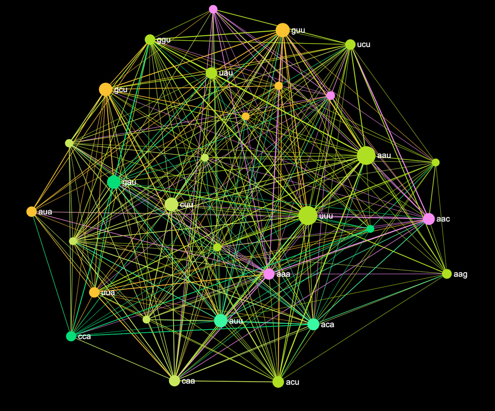
#cuu #guu We then copy and paste this into InfraNodus (feel free to try it yourself!), which will visualize every codon-hashtag as a node and every line where they co-occur as an edge in a network graph. It will look something like this:
Another interesting approach is to use that RNA sequence to build a graph of the amino acids that will be produced. So instead of visualizing the codons, we will transcribe every codon into the amino acid that is made from it, and represent the graph in this way.
So, for the sample codon sequence above:
#aug #uuu
#uuu #guu
#guu #uuu
#uuu #cuu
#cuu #guu
becomes the amino acids sequence:
#Methionine #Phenylalanine
#Phenylalanine #Valine
#Valine #Phenylalanine
#Phenylalanine #Leucine
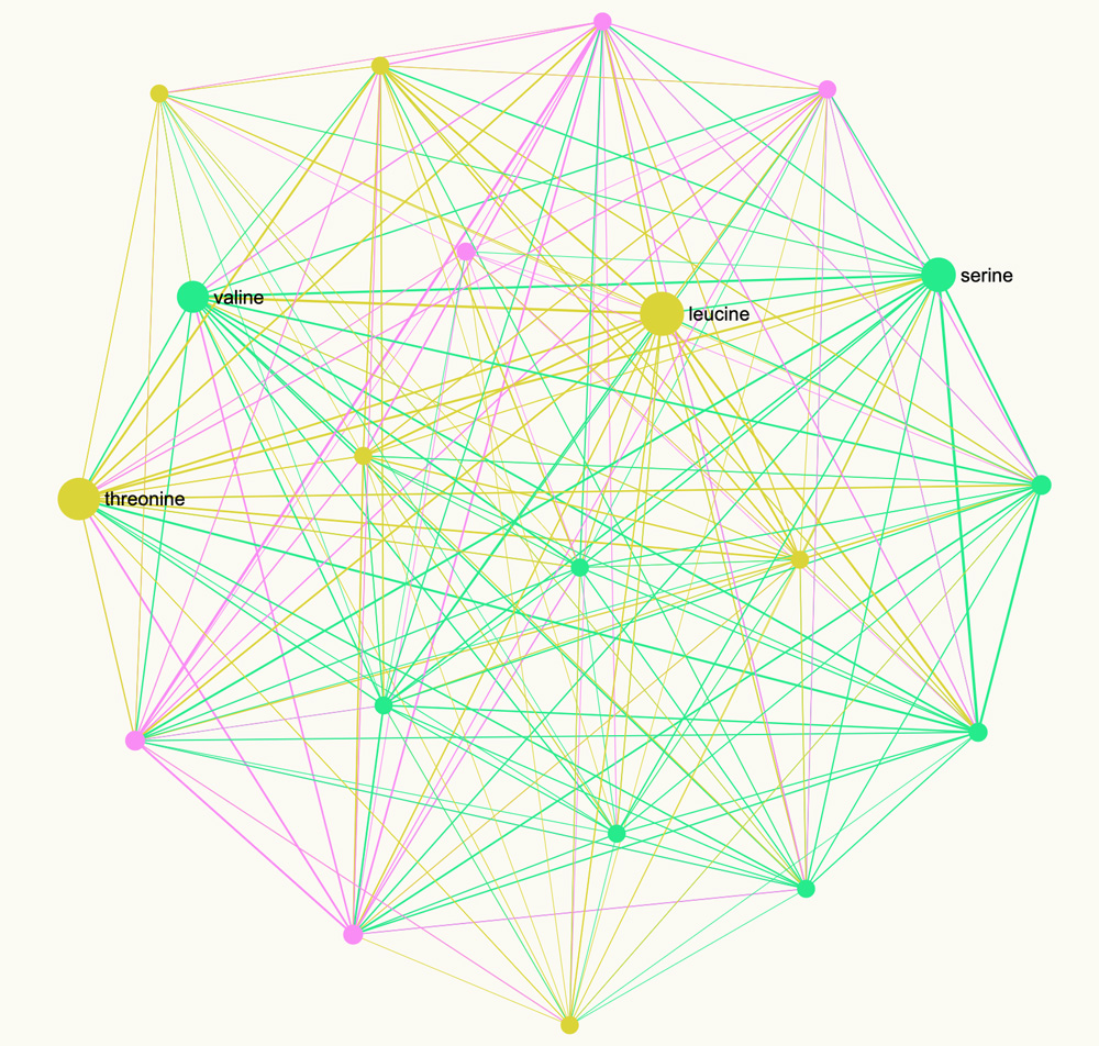
#Leucine #Valine It is important to note that such representation will decrease the dimensionality of the graph because there are 20 amino acids made out of 64 codons. So it may be interesting to also do the translation of each sequence into the graph of amino acids that can actually be produced from them:
2. How to Read the Network Graph of a Genetic Code
The graphs above shows a network graph representation of the RNA sequence for the Spike protein of coronavirus.
In order to interpret the graphs, we need to calibrate some of the basic concepts we’re going to use for our reading.
The nodes that are shown bigger on the graph have a higher measure of betweenness centrality. Betweenness centrality is often used as a measure of influence showing how often a node appears on the shortest path between any other two randomly chosen nodes in the network. The higher this measure is, the more connected the node is to every other node in the structure. In the context of the genetic code it means that a codon (or an amino acid, depending on the graph) with high betweenness centrality is going to appear more frequently before and after completely different sets of codons (aminoacids), linking the distinct different groups of codons that tend to co-appear together.
Betweenness centrality is not the same thing as the frequency. A codon may appear frequently in a sequence and, therefore, have a high degree (number of connections). But another codon with less connections may have a higher betweenness centrality if it appears next to a more diverse range of other codons.
Another important measure is the community structure of the graph. The nodes will be aligned closer to each other on the graph and have the same color if they are more densely connected together than with the rest of the network.
InfraNodus‘ statistical tools provide the insight about these both measures:

From this data we can see that the most “influential” codons (high betweenness centrality) in this sequence are the
uuu aau guuWhile the ones that tend to co-occur together are:
1: uuu  aau  acu
2: gcu  guu  uua
3: caa  gaa  cuu
4: auu  aca  ggc
This gives us an interesting structural insight about this sequence, revealing some patterns within. We can use this insight to identify similarities between the different proteins, get a deeper understanding of how they work, and understand what may be the crucial elements that are involved in the replication process.
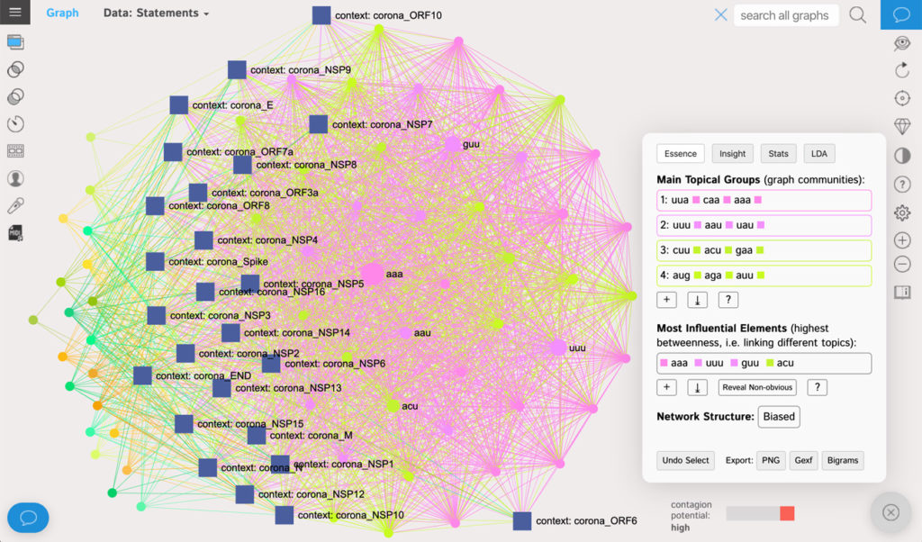
For example, if we create a separate graph for each of the proteins in the Coronavirus sequence and then put them all together, we will get an aggregate graph, which will show not only which codons tend to be more “influential” in network terms, but also — which of them tend to belong together and how the proteins can be categorized depending on their connectivity structure:
(open the full-screen interactive on InfraNodus)
Using the graph and the network analytics provided by InfraNodus we can reveal some interesting patterns in the structure virus’ proteins.
First, the codons with the highest betweenness centrality (and thus, influence) among all the proteins are:
aaa uuu guu acuLooking closer at the Statistics table in the Analytics panel (see the CSV file with the codon network data) we will see some interesting discrepancies.
For instance, when the codons are sorted by frequency as below, we can see that uuu has a slightly lower frequency but a higher betweenness centrality measure than the others in the top 16 list (relatively high bc / freq ratio — conductivity). That means that those this codon is a “connector” and appears more often in very different sequences of codons. So it could be an especially crucial element in the structure of the virus even though it’s not the most frequent one.
At the same time, we can also see that ggu is an outlier, because unlike its neighbors from the most connected nodes list it has a very high degree to betweenness centrality ratio (what we call locality). Which means that it tends to appear more often with a certain group of specific codons. Interestingly, it does not appear neither in ORF6, nor in ORF10 proteins.
| node | degree | freq | bc | bc / degree | degree / bc | bc / freq |
| aaa | 110 | 755 | 0.220377 | 20.0 | 5 | 2.9 |
| guu | 110 | 740 | 0.107973 | 9.8 | 11 | 1.5 |
| aau | 111 | 709 | 0.037652 | 3.4 | 33 | 0.5 |
| gcu | 108 | 702 | 0.028793 | 2.7 | 41 | 0.4 |
| uuu | 111 | 700 | 0.121262 | 10.9 | 10 | 1.7 |
| ggu | 109 | 650 | 0.003322 | 0.3 | 358 | 0.1 |
| acu | 111 | 636 | 0.056478 | 5.1 | 22 | 0.9 |
| gau | 110 | 620 | 0.016611 | 1.5 | 73 | 0.3 |
| gaa | 110 | 604 | 0.020487 | 1.9 | 59 | 0.3 |
| aca | 110 | 589 | 0.028239 | 2.6 | 43 | 0.5 |
| uau | 110 | 546 | 0.024363 | 2.2 | 50 | 0.4 |
| cuu | 112 | 538 | 0 | 0.0 | 0 | 0.0 |
| uua | 111 | 514 | 0.019934 | 1.8 | 62 | 0.4 |
| auu | 107 | 512 | 0.006645 | 0.6 | 172 | 0.1 |
| caa | 110 | 492 | 0.003322 | 0.3 | 364 | 0.1 |
| ugu | 105 | 458 | 0.003322 | 0.3 | 332 | 0.1 |
We can also look at the table of bigrams (below — CSV download), from which we will see that the codon ggu is often followed by guu. Considering that we identified guu earlier as a codon of global importance (high BC), while ggu was identified as a codon of local importance (high degree to BC ratio), we can discern that ggu may be the point of transition from some sort of specificity in the sequence to a more generic pattern.
| from | to | weight |
| ggu | guu | 87 |
| ggu | gau | 72 |
| gcu | gcu | 66 |
| gcu | ggu | 63 |
| gaa | gaa | 63 |
| gcu | guu | 60 |
| gau | gcu | 57 |
| ugu | guu | 57 |
| guu | guu | 57 |
| aau | ggu | 57 |
| acu | aau | 57 |
| aau | guu | 57 |
We can then remove the periphery of the graph or the codons that are not connected to any other significant codons in the graph and only have local importance, to see how the proteins will align themselves in relation to the overall mass. The alignment follows force-atlas algorithm, which pulls together the nodes that are better connected and pushes the most connected nodes apart:

We can compare these relations between the proteins to the descriptions of their functions and compare whether there is correlation between the most influential codons and the functional similarities of the different proteins they comprise.
We can further click “reveal the non-obvious” button to see the other influential elements behind the ones that we identified already in order to find more patterns within.
The next step is to look at every protein network structure separately in order to find the similarities and discrepancies in the structure among them.
Finally, the same graphs can be built for amino acids that can be produced by those codons as this may reduce dimensionality of the analysis and reveal some interesting patterns at the level of transcription.
We will be updating this article as we go more in-depth in this analysis.
Try it yourself… and — to be continued!
We have demonstrated above a method for representing the RNA / DNA sequences as a network graph where the nodes are the codons and their co-occurrences are the relations between them.
Below we provide an interactive visualization of the proteins found in the virus (see the New York Times Interactive by Carl Zimmer and Jonathan Corum). You can play around with it, using the menu in the top left to switch between the different protein graphs (the Spike S protein is loaded by default). You can also open it in a new window to have a bit more space to work with.
This representation is still at a very experimental stage. However, we think it can yield especially interesting results if we start comparing the different types of RNA or the structures of the different proteins.
For instance, there may be some similarities between the different viruses. Certain codons and certain structural patterns of their organization in may be related to certain protein function. The same analysis performed on amino acids may also reveal interesting results.
We encourage you to try the tools that we created to continue the research in this direction and to share it with us on Twitter using the @noduslabs and #infranodus so we can help you spread it further.
• InfraNodus network visualization and analysis platform
• RNA nucleotides to codon sequence convertor (modify the code for DNA)
• original datasets from the NYTimes Interactive
Also, please, let us know if you have any ideas or feedback. We will be happy to hear from you or to help you with your research!
Bonus Track: Alternative Encodings
The above representation have shown the most practical way of encoding an RNA or a DNA sequence: representing the codons or amino acids as the nodes and their co-occurrences as the connections. This is the way RNA transcription operates, so in the context of Coronavirus it makes sense.
However, there could be different ways of representing the nucleotide sequence, which may be not so interesting from a practical perspective, but reveal an interesting approach that could be used in other contexts.
For example, we could represent the RNA sequence itself as a network, where the nucleotides or as the nodes and their co-occurrences as the edges in the network (using this this one to one RNA converter). Using the Spike protein sequence of Coronavirus we will get this graph:
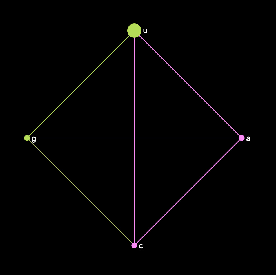
From this graph we can see that Uracil is quite prominent in this sequence and that U and G tend to occur more often together, while A and C belong to another cluster. We can also see that C and G tend to occur less often than other combinations.
We can also retrieve the table of bigrams from InfraNodus analytics panel to see which combinations tend to occur more often. The excerpt is below:
| from | to | weight |
| u | u | 1398 |
| a | a | 1098 |
| u | g | 987 |
| a | u | 909 |
| c | a | 909 |
| u | a | 798 |
| c | u | 795 |
U and A are the most prominent elements but U appears more often as the connector to other nucleobases, so it has a higher influence (betweenness centrality) in this sequence.
Now, let’s say we wanted to see which combinations of nucleotides occur more often. This may be meaningless in the field of biology, but as an abstract exercise it provides an interesting way of representing a sequence, similar to what differential equations do in the field of calculus. For example, if we take this succession of nucleotides:
c → c → u → c → g → g → c → g → g → g → c → a… and convert them into pairs (so, first it’s cc that occurs, then it’s cu, then it’s uc and so on — using this converter to pairs), we would get this:
cc → cu
cu → uc
uc → cg
cg → gg
gg → gc
gc → cg
cg → gg
gg → gg
gg → gc
gc → ca
Now, if we translate the same way the long sequence of the S Spike protein from above, we will get this graph:
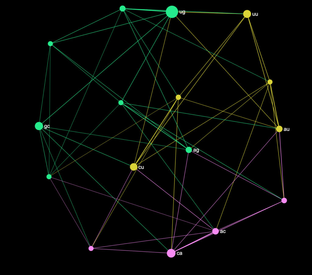
The analytics panel of InfraNodus shows us that the most influential pairs of nucleobases are:
U → G | C → A | G → C | U → UThis is in contrast to the most prominent bigrams shown earlier (UU, AA, UG). The reason is that while the combination of UU appears 344 times and the combination UG appears 329 times (slightly less frequent), UG will appear more often as a link between the different clusters of nucleobase sequences in this protein.

We can also see that there are several clusters of pairs formed:
1: U → G | G → U | G → G
2: U → U | U → C | U → A
3: C → C | C → A | A → C
This indicates that those pairs tend to occur more often in the same context in this protein.